Linear Least Squares
Suppose that you have \(n\) data points \((x_i, y_i)\) which were generated by a model \(y = f(x) + \epsilon\), where \(\epsilon\) is an error term given by a normal distribution. If you know \(f(x)\) up to a linear combination of parameters, then the linear least squares (LLS) method can find values for them so that the model fits the data.
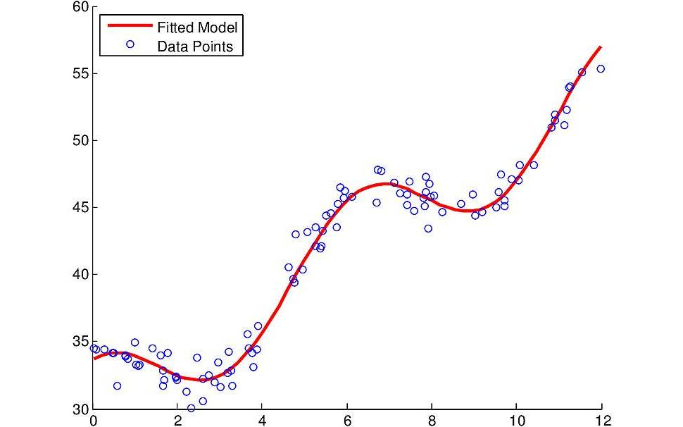
As an example, the above figure shows some noisy data points taken from the model
\[f(x) = a x + b \cos(x) + c,\]in which \((a, b, c)\) are unknown constants. To find their values from the data, we can build a matrix \(\mathbf{A}\) and a vector \(\mathbf{b}\) such that
\[\mathbf{A} = \begin{bmatrix} x_1 & \cos(x_1) & 1 \\ x_2 & \cos(x_2) & 1 \\ & \vdots & \\ x_n & \cos(x_n) & 1 \\ \end{bmatrix} \;\;\; \mathbf{b} = \begin{bmatrix} y_1 \\ y_2 \\ \vdots \\ y_n \end{bmatrix},\]and together with the parameter vector \(\mathbf{x} = [a, b, c]^T\), the problem can be reduced to finding the solutions of the linear system \(\mathbf{Ax} = \mathbf{b}\).
It is likely that matrix \(\mathbf{A}\) is non-square, as we expect to have more data points available (rows) than unknown parameters (columns), namely an overdetermined system. Otherwise, we could just invert \(\mathbf{A}\) to find the unique solution \(\mathbf{x} = \mathbf{A}^{-1}\mathbf{b}\). As this is not possible, we need another approach.
The Algebraic Approach
By left-multiplying matrix \(\mathbf{A}^T\) on both sides of \(\mathbf{Ax} = \mathbf{b}\), we have
\[(\mathbf{A}^T\mathbf{A})\mathbf{x} = \mathbf{A}^T \mathbf{b}.\]And because \(\mathbf{A}\) is composed of linearly independent columns, the square matrix \(\mathbf{A}^T\mathbf{A}\) is invertible (proof). Hence, the solution to the linear system is simply given by
\[\mathbf{x} = (\mathbf{A}^T\mathbf{A})^{-1} \mathbf{A}^T \mathbf{b}.\]The simplicity of this solution does not bring any mathematical insights, and hence I do not consider it as particularly interesting. A more insightful approach can be found by delving into the theory of Linear Algebra.
The Insightful Approach
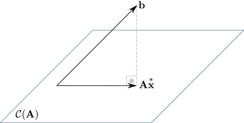
As there is no solution to the system \(\mathbf{Ax} = \mathbf{b}\) then we can conclude that \(\mathbf{b}\) does not belong to the column space \(\mathcal{C}(\mathbf{A})\) of matrix \(\mathbf{A}\). In this manner, we could instead look for a vector \(\overset{*}{\mathbf{x}}\) so that \(\mathbf{A}\overset{*}{\mathbf{x}}\) is the nearest vector to \(\mathbf{b}\) according to the Euclidean metric. Formally, we want to compute
\[\overset{*}{\mathbf{x}} = \underset{\mathbf{x}}{\arg\min} \lVert \mathbf{Ax} - \mathbf{b} \rVert.\]Note that computing the square root in the Euclidean norm is not necessary. The solution will be exactly the same because the square root is a monotonic function. This is why the method is called Least Squares: each element of \(\mathbf{Ax - b}\) is squared and summed together, and the vector \(\mathbf{x}\) that results in the least amount of residual error in relation to \(\mathbf{b}\) is the solution \(\overset{*}{\mathbf{x}}\).
One way of finding \(\overset{*}{\mathbf{x}}\) is to realize that \(\mathbf{A}\overset{*}{\mathbf{x}}\) must be the orthogonal projection of \(\mathbf{b}\) onto \(\mathcal{C}(\mathbf{A})\) (proof). Hence, the vector \(\mathbf{A}\overset{*}{\mathbf{x}} - \mathbf{b}\) must be perpendicular to \(\mathbf{A}\overset{*}{\mathbf{x}}\), which means that the former must belong to the null space of \(\mathbf{A}^T\), as this space is the orthogonal complement of \(\mathcal{C}(\mathbf{A})\).
By definition, any vector belongs to the null space of a matrix when the former is mapped onto the zero vector by the latter. Given the discussion at the previous paragraph, we must have
\[\begin{align*} \mathbf{A}^T (\mathbf{A}\overset{*}{\mathbf{x}} - \mathbf{b}) &= \mathbf{0} \\ \mathbf{A}^T \mathbf{A}\overset{*}{\mathbf{x}} - \mathbf{A}^T \mathbf{b} &= \mathbf{0} \\ \mathbf{A}^T \mathbf{A}\overset{*}{\mathbf{x}} &= \mathbf{A}^T \mathbf{b}, \end{align*}\]in which we can invert \(\mathbf{A}^T\mathbf{A}\) because of the same reasons as in the prior section. This leads us to the expected solution
\[\overset{*}{\mathbf{x}} = (\mathbf{A}^T \mathbf{A})^{-1}\mathbf{A}^T \mathbf{b}.\]A Numerical Stable Solution to LLS
Because of numerical instabilities in floating point arithmetic, computing \((\mathbf{A}^T \mathbf{A})^{-1}\mathbf{A}^T \mathbf{b}\) is not a wise decision. A better approach is to apply the QR decomposition algorithm to break down matrix \(\mathbf{A}\) into two matrices: \(\mathbf{Q}\), an orthogonal matrix, and \(\mathbf{R}\), an upper-triangular matrix, such that \(\mathbf{A} = \mathbf{QR}\). I won’t go through the details of the algorithm, but a simple method is to find \(\mathbf{Q}\) by applying the Gram-Schmidt process and then to compute \(\mathbf{R} = \mathbf{Q}^T \mathbf{A}\). After the decomposition, we can easily find another way of computing \(\overset{*}{\mathbf{x}}\) as follows.
\[\begin{align*} \overset{*}{\mathbf{x}} &= (\mathbf{A}^T \mathbf{A})^{-1}\mathbf{A}^T \mathbf{b} \\ \overset{*}{\mathbf{x}} &= ((\mathbf{QR})^T \mathbf{QR})^{-1}(\mathbf{QR})^T \mathbf{b}\\ \overset{*}{\mathbf{x}} &= (\mathbf{R}^T\mathbf{Q}^T \mathbf{QR})^{-1}\mathbf{R}^T\mathbf{Q}^T \mathbf{b}\\ \overset{*}{\mathbf{x}} &= (\mathbf{R}^T \mathbf{R})^{-1}\mathbf{R}^T\mathbf{Q}^T \mathbf{b}\\ \overset{*}{\mathbf{x}} &= \mathbf{R}^{-1}\mathbf{Q}^T \mathbf{b}\\ \mathbf{R} \overset{*}{\mathbf{x}} &= \mathbf{Q}^T \mathbf{b} \end{align*}\]The last equation can easily be solved by the back substitution algorithm, and the result is more numerically stable than the direct computation.