Exponential Smoothing

I did a lot of bug fixing in legacy code that uses the Unity Engine, and I noticed an odd pattern being used for moving GameObjects towards a target position.

transform.position = Vector3.Lerp(transform.position, targetPosition, Time.deltaTime);

The code makes the object start moving at a high speed while smoothly decelerating until reaching the target. The movement is interesting and many Unity developers seem to like it, even though some of them do not completely understand why it works. It is even used in the official tutorial of Vector3.Lerp. Despite its simplicity, this line of code has some issues.

• The intent is not clear: the code seems to be doing a proper linear interpolation, but the resulting movement is nonlinear.
• Framerate dependency: if a machine can run the game loop faster, then it will reach the target position in less time.
• Reliance on floating-point error: the target is only reached because of precision loss in floating-point arithmetic.

Fortunately, the solution to these problems is simple: the value of the third parameter must be adjusted using a power function based on Time.deltaTime and a constant epsilon, which specifies an acceptable radius for reaching the target.

float t = 1.0f - Mathf.Pow(epsilon, Time.deltaTime);
transform.position = Vector3.Lerp(transform.position, targetPosition, t);

The following sections explain why this is a proper solution by exploring the mathematics of this particular usage of Vector3.Lerp, which is known as exponential smoothing.

Linear Interpolation and Exponential Smoothing

Vector3.Lerp computes a linear interpolation between two vectors \(\mathbf{A}\) and \(\mathbf{B}\) and can be described as

\[\mathit{Lerp}(\mathbf{A}, \mathbf{B}, t) = (1 - t)\mathbf{A} + t \mathbf{B}, \quad t \in [0,1].\]

Exponential smoothing consists in consecutive applications of Lerp in a recursive fashion. For instance, by defining \(\mathbf{p}_i\) as the i-th iteration of Lerp, the sequence

\[\begin{align*} \mathbf{p}_1 &= \mathit{Lerp}(\mathbf{A}, \mathbf{B}, t)\\ \mathbf{p}_2 &= \mathit{Lerp}(\mathbf{p}_1, \mathbf{B}, t)\\ \mathbf{p}_3 &= \mathit{Lerp}(\mathbf{p}_2, \mathbf{B}, t)\\ &\vdots\\ \mathbf{p}_n &= \mathit{Lerp}(\mathbf{p}_{n-1}, \mathbf{B}, t)\\ \end{align*}\]

represents these consecutive, recursive applications. A natural question arises: what is the value of \(\mathbf{p}_n\)? We can answer by expanding the sequence as follows.

\[\begin{align*} \mathbf{p}_1 &= (1-t) \mathbf{A} + t \mathbf{B} \\ \mathbf{p}_2 &= (1-t)^2 \mathbf{A} + (1-t)t \mathbf{B} + t \mathbf{B} \\ \mathbf{p}_3 &= (1-t)^3 \mathbf{A} + (1-t)^2t \mathbf{B} + (1-t)t \mathbf{B} + t \mathbf{B} \\ \vdots& \\ \mathbf{p}_n &= (1-t)^n \mathbf{A} + \left[ \sum_{i=0}^{n-1}(1-t)^i\right] t \mathbf{B} \end{align*}\]

The above summation is a geometric series whose solution is

\[\sum_{i=0}^{n-1}(1-t)^i = \frac{1 - (1-t)^n}{t},\]

which, assuming \(t \neq 0\), let us write a direct formula for the n-th iteration as

\[\mathbf{p}_n = (1-t)^n \mathbf{A} + (1 - (1-t)^n) \mathbf{B}.\]

By defining \(u = 1 - t\), the equation can be simplified to

\[\mathbf{p}_n = u^n \mathbf{A} + (1 - u^n) \mathbf{B}.\]

Notice how the formula resembles linear interpolation, but instead of using linear blending functions \(t\) and \((1-t)\), we use exponential blending functions \((1-u^n)\) and \(u^n\). This is why the technique is called exponential smoothing.

Zeno’s Paradox

We can rewrite \(\mathbf{p}_n\) in terms of a single exponential function as

\[\mathbf{p}_n = \mathbf{B} + u^n (\mathbf{A}-\mathbf{B}),\]

which makes it clear that \(\mathbf{B}\) is reached as \(u^n\) approaches zero. If we take \(u=0.5\) then the first five elements of the sequence are

\[\begin{align*} \mathbf{p}_1 &= \mathbf{B} + 0.5^1(\mathbf{A} - \mathbf{B}) = 0.5\mathbf{A} + 0.5\mathbf{B}\\ \mathbf{p}_2 &= \mathbf{B} + 0.5^2(\mathbf{A} - \mathbf{B}) = 0.25\mathbf{A} + 0.75\mathbf{B}\\ \mathbf{p}_3 &= \mathbf{B} + 0.5^3(\mathbf{A} - \mathbf{B}) = 0.125\mathbf{A} + 0.875\mathbf{B}\\ \mathbf{p}_4 &= \mathbf{B} + 0.5^4(\mathbf{A} - \mathbf{B}) = 0.0625\mathbf{A} + 0.9375\mathbf{B}\\ \mathbf{p}_5 &= \mathbf{B} + 0.5^5(\mathbf{A} - \mathbf{B}) = 0.03125\mathbf{A} + 0.96875\mathbf{B}. \end{align*}\]

The sequence quickly converges towards the target point but at an ever slowing pace. In fact, we will only reach \(\mathbf{B}\) after infinitely many iterations. This pattern is one of the three paradoxes of motion by Zeno, a greek philosopher and mathematician.

Framerate Independence

To control the movement speed, we need to command the rate at which \(u^n\) approaches zero. Also, we want it to be consistent across different framerates.

Let \(\epsilon\) be the radius of a small sphere centered at the target. When the sphere is reached we will instead assume that the target is reached up to an error bound \(\epsilon\). Naturally, we should seek a value \(u\) so that after \(n\) iterations \(u^n\) is exactly \(\epsilon\). This can be done by setting \(u = \sqrt[n]{\epsilon}\) (hence \(t = 1 - \sqrt[n]{\epsilon})\).

The plot below displays the behaviour of exponential smoothing given \(\epsilon = 0.5\) and \(n = 30\). As it can be seen, \(\epsilon\) is reached at 30 iterations, \(\epsilon^2\) at 60 iterations, and so on. This means that if your game is running at 30 FPS, then half the distance between \(\mathbf{A}\) and \(\mathbf{B}\) will be reached in one second, a quarter in two seconds, and so on.

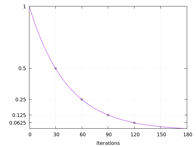
Now suppose that your game is running at 60 FPS, and you are using the same values for \(n\) and \(\epsilon\). Now, half the distance will be reached in a half second. This is inconsistent when compared to the same game running at 30 FPS. In order to correct the issue you must set \(n = 60\). In the general case, \(n\) should be set to the current FPS at which your game is running.

In the Unity Engine, we can approximate the current FPS by using the delta time between frames, which means that we can simply set \(n = \frac{1}{\Delta T}\). This inverse relation is interesting because it turns the n-th square root in \(t = 1 - \sqrt[n]{\epsilon}\) into the n-th power

\[t = 1 - \epsilon^{\Delta T}.\]

The final code is just a translation of the above formula, as already presented in the first section.

float t = 1.0f - Mathf.Pow(epsilon, Time.deltaTime);
transform.position = Vector3.Lerp(transform.position, targetPosition, t);